
All experiments were run using custom-written code for the Python machine learning framework PyTorch65.
Context sets
For the Split MNIST protocol, the MNIST dataset66 was split into five contexts, such that each context contained two digits. The digits were randomly divided over the five contexts, so the order of the digits was different for each random seed. The original 28×28 pixel greyscale images were used without pre-processing. The standard training/test-split was used, which resulted in 60,000 training images (approximately 6,000 per digit) and 10,000 test images (approximately 1,000 per digit).
For the Split CIFAR-100 protocol, the CIFAR-100 dataset67 was split up into ten contexts, such that each context contained ten image classes. The classes were randomly divided over the contexts, with a different class order for each random seed. The original 32×32 pixel RGB-colour images were normalized (that is, each pixel-value was subtracted by the relevant channel-wise mean and divided by the channel-wise standard deviation, with means and standard deviations calculated over all training images). No other pre-processing or augmentation was applied. The standard training/test-split was used, which resulted in 50,000 training images (500 per class) and 10,000 test images (100 per class).
Base neural network architecture
To make the comparisons as informative as possible, we used the same base neural network architecture for all methods as much as possible. For Split MNIST, the base network had two fully connected hidden layers of 400 ReLU each and a softmax output layer. For Split CIFAR-100, the base network had five pre-trained convolutional layers followed by two fully connected layers with 2,000 ReLU each and a softmax output layer. The convolutional layers contained 16, 32, 64, 128 and 256 channels. Each convolutional layer used a 3×3 kernel, a padding of 1 and there was a stride of 1 in the first layer (that is, no downsampling) and a stride of 2 in the other layers (that is, image-size was halved in each of those layers). Batch norm68 was used in all convolutional layers, followed by a ReLU non-linearity. No pooling was used. The convolutional layers were pre-trained on CIFAR-10, which is a dataset containing similar but non-overlapping images and image classes compared with CIFAR-10067. To pre-train the convolutional layers, the base neural network was trained to classify the 10 classes of CIFAR-10 for 100 epochs, using the ADAM-optimizer (β1 = 0.9, β2 = 0.999) with learning rate of 0.0001 and mini-batch size of 256. For the pre-training on CIFAR-10, images were normalized and augmented by random cropping and horizontal flipping. A similar pre-training protocol was used in ref. 28. During the incremental training on CIFAR-100, the parameters of the pre-trained convolutional layers were frozen. For all compared methods, freezing these parameters resulted in similar or better performance compared with not freezing them.
Output layer
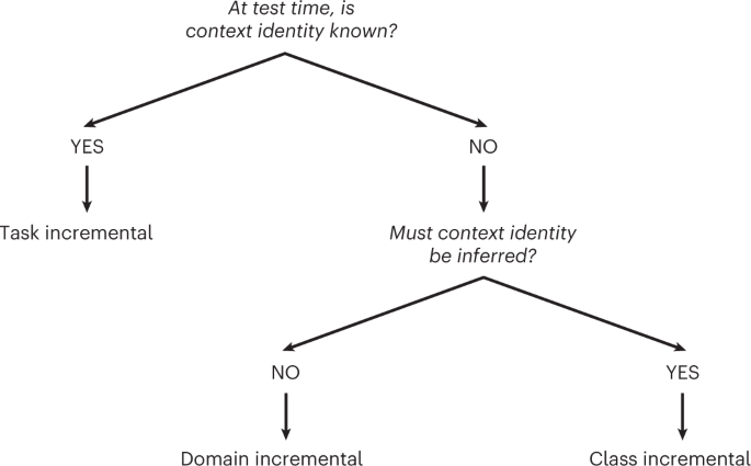
The softmax output layer of the network was treated differently depending on the continual learning scenario that was performed. With task-incremental learning, a multi-headed output layer was used, meaning that each context had its own output units and only the output units of the context under consideration—that is, either the current context or the replayed context—were set to ‘active’ (see next paragraph). With domain- and class-incremental learning, a single-headed output layer was used. For domain-incremental learning, this meant that all contexts used the same output units (that is, there were 2 output units for Split MNIST and 10 for Split CIFAR-100); for class-incremental learning, this meant that each class had its own output unit (that is, there were 10 output units for Split MNIST and 100 for Split CIFAR-100). With both domain- and class-incremental learning, always all output units were set to ‘active’. Note that with class-incremental learning another possibility is to use an ‘expanding head’ and only set the output units of classes seen so far to active (for example, see refs. 28,69). We found that for our experiments there was not much difference in performance between these two options. Because all output units should always be active for the Bayesian interpretation of the parameter regularization methods21, we decided to use that approach in this study.
Whether an output unit was set to ‘active’ controlled whether a network could assign a positive probability to its corresponding class. The probability predicted by a neural network with parameters θ that an input x belongs to output class o was calculated as:
$${p}_{{{{{theta }}}}}left(o| {{{{x}}}}right)=left{begin{array}{ll}frac{{e}^{{z}_{o}^{({{{{x}}}},{{{{theta }}}})}}}{{sum }_{j}{e}^{{z}_{j}^{({{{{x}}}},{{{{theta }}}})}}}quad &{{{rm{if}}}},{{{rm{output}}}},{{{rm{unit}}}},o,{{{rm{is}}}},{{{rm{active}}}}\ {{{rm{0}}}}quad &{{{rm{otherwise}}}}end{array}right.$$
(2)
whereby ({z}_{o}^{({{{{x}}}},{{{{theta }}}})}) was the logit of output class o obtained by putting input x through the neural network with parameters θ. The summation in the denominator was over all active classes in the output layer. Importantly, with task- and class-incremental learning, output class o refers to the ‘global class’ that is obtained by combining the within-context label y and the context label c (that is, the set of global classes is given by ({{{mathcal{G}}}}={{{mathcal{Y}}}}times {{{mathcal{C}}}})). With domain-incremental learning, output class o refers to the within-context label y.
Data stream
All experiments in this article used the academic continual learning setting, meaning that the different contexts were presented to the algorithm one after the other. Within each context, the training data was fed to the algorithm in a stream of independent and identically distributed experiences (or iterations). For Split MNIST, each context was trained for 2,000 iterations with mini-batch size of 128. For Split CIFAR-100, there were 5,000 iterations per context with mini-batch size of 256. Some of the compared methods (EWC, FROMP and iCaRL) performed an additional pass over each context’s training data upon finishing training on that context.
Loss function and optimization
For all compared methods, the parameters of the neural network were sequentially trained on each context by optimizing a loss function (denoted by ({{{{mathcal{L}}}}}_{{{{rm{total}}}}})) using stochastic gradient descent. In each iteration, the loss was calculated as the average over all samples in the mini-batch and a single gradient step was taken with the ADAM-optimizer (β1 = 0.9, β2 = 0.999; ref. 70) and a learning rate of either 0.001 (Split MNIST) or 0.0001 (Split CIFAR-100).
For most compared methods, a central component of the loss function was the multi-class cross-entropy classification loss on the data of the current context. For an input x labeled with a hard target o, this classification loss was given by:
$${{{{mathcal{L}}}}}^{{{{rm{C}}}}}left({{{{x}}}},o;{{{{theta }}}}right)=-log {p}_{{{{{theta }}}}}left(o| {{{{x}}}}right)$$
(3)
with pθ the conditional probability distribution defined by the neural network with parameters θ, as given in equation (2).
Memory buffer and generative models
Several of the compared methods (FROMP, ER, A-GEM and iCaRL) maintained a memory buffer in which examples of previously seen classes were stored. Except for the experiments in Extended Data Fig. 1, 100 examples per class were allowed to be stored in the memory buffer (that is, the per-class memory budget B was set to 100). Some other methods (DGR, BI-R and the Generative Classifier) learned generative models, these methods used up to three times as many parameters compared with the other methods.
Baselines
For the baseline ‘None’, which was included as a lower target, the base neural network was sequentially trained on each context in the standard way, meaning that the loss function to be optimized was always just the classification loss on the current data (that is, ({{{{mathcal{L}}}}}_{{{{rm{total}}}}}={{{{mathcal{L}}}}}^{{{{rm{C}}}}})).
For the baseline ‘Joint’, which was included as an upper target, the base neural network was trained on the data from all contexts at the same time. For this baseline, the same total number of iterations was used as with the sequential training protocol (that is, 5×2,000 iterations for Split MNIST and 10×5,000 iterations for Split CIFAR), but each mini-batch was always sampled jointly from the data of all contexts.
Approaches using context-specific components
For XdG and the ‘Separate Networks’ approach, not all parts of the network were used for each context. These approaches require knowledge of which context a sample belongs to (to select the correct context-specific components), which meant that they could only be used in the task-incremental learning scenario. For both approaches, training was performed using just the classification loss on the current data (that is, ({{{{mathcal{L}}}}}_{{{{rm{total}}}}}={{{{mathcal{L}}}}}^{{{{rm{C}}}}})).
In the task-incremental learning scenario, the other methods (that is, all methods except XdG and Separate Networks) used the available context identity information only in the form of a separate output layer for each context. This is a common and often sensible way to use context identity information, although in Supplementary Note 7 we show that sometimes it is more efficient to use context identity information in other ways.
Separate Networks
For the Separate Networks approach, the available parameter budget was equally divided over all contexts to be learned, and a separate sub-network was trained for each context. For Split MNIST, each context-specific sub-network had two fully connected hidden layers of 100 ReLU each and a softmax output layer. For Split CIFAR-100, the pre-trained and frozen convolutional layers were shared between all contexts, and only the fully connected part of the network was split up into context-specific sub-networks. Each context-specific sub-network had two fully connected layers with 400 ReLU each and a softmax output layer.
XdG
With XdG12, the base neural network was used and for each context a different, randomly selected subset of X% of the units in each hidden layer was fully gated (that is, their activations were set to zero), with X a hyperparameter whose value was set by a grid search (Supplementary Note 8).
Parameter regularization methods
For the parameter regularization methods EWC and SI, a regularization term was added to the classification loss: ({{{{mathcal{L}}}}}_{{{{rm{total}}}}}={{{{mathcal{L}}}}}^{{{{rm{C}}}}}+{{{{mathcal{L}}}}}_{{{{rm{param-reg}}}}}). This regularization term penalized changes to parameters thought to be important for previously learned contexts.
EWC
The regularization term of EWC49 consisted of a quadratic penalty term for each previously learned context, whereby the term of each context penalized parameters for how different they were compared to their value directly after finishing training on that context. When training on context K > 1, the EWC regularization term was given by:
$${{{{mathcal{L}}}}}_{{{{rm{param-reg}}}}}^{(K)}left({{{{theta }}}}right)=lambda mathop{sum }limits_{k=1}^{K-1}left(frac{1}{2}mathop{sum }limits_{i=1}^{{N}_{{{{rm{params}}}}}}{F}_{ii}^{(k)}{left({theta }_{i}-{hat{theta }}_{i}^{(k)}right)}^{2}right)$$
(4)
with λ a hyperparameter controlling the regularization strength (which was set based on a grid search, Supplementary Note 8), ({hat{theta }}_{i}^{(k)}) the value of the ith parameter at the end of training on context k, and ({F}_{ii}^{(k)}) the estimated importance of parameter i for context k. This importance estimate was calculated as the ith diagonal element of the Fisher information matrix of context k:
$${F}_{ii}^{(k)}=frac{1}{| {S}^{(k)}| }mathop{sum}limits_{{{{{x}}}}in {S}^{(k)}}left(mathop{sum}limits_{o}{hat{o}}_{k}^{left({{{{x}}}}right)}{left({left.frac{delta log {p}_{{{{{theta }}}}}left(o| {{{{x}}}}right)}{delta {theta }_{i}}right|}_{{{{{theta }}}} = {hat{{{{{theta }}}}}}^{(k)}}right)}^{2}right)$$
(5)
whereby S(k) was the training data of context k and ({hat{o}}_{k}^{left({{{{x}}}}right)}) was the probability that x belongs to output class o, as predicted by the network after finishing training on context k—that is, ({hat{o}}_{k}^{left({{{{x}}}}right)}={p}_{{hat{{{{{theta }}}}}}^{(k)}}left(o| {{{{x}}}}right)). The inner summation in equation (5) was over all output classes that were active during training on context k.
SI
The regularization term of SI (ref. 31) consisted of a single quadratic term that penalized changes to the parameters away from the value they had after finishing training on the previous context. When training on context K > 1, the SI regularization term was given by:
$${{{{mathcal{L}}}}}_{{{{rm{param-reg}}}}}^{(K)}left({{{{theta }}}}right)=gamma mathop{sum }limits_{i=1}^{{N}_{{{{rm{params}}}}}}{{{Omega }}}_{i}^{(K-1)}{left({theta }_{i}-{hat{theta }}_{i}^{* }right)}^{2}$$
(6)
with γ a hyperparameter controlling the regularization strength (which was set based on a grid search, see Supplementary Note 8), ({hat{theta }}_{i}^{* }) the value of the ith parameter at the end of training on context K − 1, and ({{{Omega }}}_{i}^{(K-1)}) the estimated importance of parameter i after the first K − 1 contexts have been learned. To compute these parameter importance estimates, after each context k, a per-parameter contribution to the change of the loss was calculated for each parameter i as follows:
$${omega }_{i}^{(k)}=mathop{sum }limits_{t=1}^{{N}_{{{{rm{iters}}}}}}left({theta }_{i}[{t}^{(k)}]-{theta }_{i}[{left(t-1right)}^{(k)}]right)frac{-delta {{{{mathcal{L}}}}}_{{{{rm{total}}}}}[{t}^{(k)}]}{delta {theta }_{i}}$$
(7)
with Niters the number of iterations per context, θi[t(k)] the value of parameter i after the tth training iteration on context k and (frac{delta {{{{mathcal{L}}}}}_{{{{rm{total}}}}}[{t}^{(k)}]}{delta {theta }_{i}}) the gradient of the loss with respect to parameter i during the tth training iteration on context k. For every context, these per-parameter contributions were normalized by the square of the total change of that parameter during training on that context plus a small dampening term ξ (set to 0.1, to bound the resulting normalized contributions when a parameter’s total change goes to zero), after which they were summed over all contexts so far:
$${{{Omega }}}_{i}^{(K-1)}=mathop{sum }limits_{k=1}^{K-1}frac{{omega }_{i}^{(k)}}{{left({{{Delta }}}_{i}^{(k)}right)}^{2}+xi }$$
(8)
with ({{{Delta }}}_{i}^{(k)}={theta }_{i}[{{N}_{{{{rm{iters}}}}}}^{(k)}]-{theta }_{i}[{0}^{(k)}]), where θi[0(k)] was the value of parameter i right before starting training on context k.
Functional regularization methods
Similar as with parameter regularization, the functional regularization methods LwF and FROMP had a regularization term added to the classification loss: ({{{{mathcal{L}}}}}_{{{{rm{total}}}}}={{{{mathcal{L}}}}}^{{{{rm{C}}}}}+{{{{mathcal{L}}}}}_{{{{rm{func-reg}}}}}). This regularization term encouraged the input–output mapping of the network not to change too much at a set of anchor points.
LwF
The method LwF (ref. 50) used the inputs from the current context as anchor points in combination with knowledge distillation71. During training on context K > 1, the LwF regularization term was given by:
$${{{{mathcal{L}}}}}_{{{{rm{func-reg}}}}}^{(K)}left({{{{x}}}},{{{{theta }}}}right)=-mathop{sum }limits_{k=1}^{K-1}mathop{sum}limits_{oin {{{{mathcal{O}}}}}_{k}}{p}_{{hat{{{{{theta }}}}}}^{* }}^{T}left(o| {{{{x}}}}right)log left[{p}_{{{{{theta }}}}}^{T}left(o| {{{{x}}}}right)right]$$
(9)
whereby ({{{{mathcal{O}}}}}_{k}) was the set of output classes in context k, ({hat{{{{{theta }}}}}}^{* }) was the parameter vector with values as they were at the end of training on context K − 1 and ({p}_{{{{{theta }}}}}^{T}left(o| {{{{x}}}}right)) was the ‘temperature-raised’ probability that input x belongs to output class o, as predicted by the network with parameters θ. These temperature-raised probabilities were defined as:
$${p}_{{{{{theta }}}}}^{T}left(o| {{{{x}}}}right)=frac{exp left[{z}_{o}^{({{{{x}}}},{{{{theta }}}})}/Tright]}{{sum }_{j}exp left[{z}_{j}^{({{{{x}}}},{{{{theta }}}})}/Tright]}$$
(10)
with T the temperature, which was set to 2, and ({z}_{o}^{({{{{x}}}},{{{{theta }}}})}) the logit of output class o obtained by putting input x through the neural network with parameters θ. The summation in the denominator was over all active classes in the output layer. With task-incremental learning, for each context’s term in the outer summation of equation (9), only the output classes contained in that context were active. With domain- and class-incremental learning, always all output classes were active. In each iteration, the LwF regularization term was computed as average over the same inputs that were used to compute ({{{{mathcal{L}}}}}^{{{{rm{C}}}}}).
We note that this implementation of LwF differs slightly from the implementation of LwF used in ref. 28. Compared with that implementation, the regularization term here was weighted less strongly, which substantially improved the performance of LwF on Split CIFAR-100. Initial experiments indicated that by reducing the weight of the replay term in equation (16) it is also be possible to improve the performance of several of the replay methods on Split CIFAR-100, but at the cost of impaired performance on Split MNIST.
FROMP
The method FROMP (ref. 51) performed functional regularization in a Bayesian framework and used stored data from previous contexts, referred to as memorable inputs, as anchor points. During training on context K, the regularization term of FROMP was given by:
$${{{{mathcal{L}}}}}_{{{{rm{func-reg}}}}}^{(K)}left({{{{theta }}}}right)=frac{1}{2}tau mathop{sum }limits_{k=1}^{K-1}mathop{sum}limits_{oin {{{{mathcal{O}}}}}_{k}}{left({{{{{m}}}}}_{k,o}^{({{{{theta }}}})}-{{{{{m}}}}}_{k,o}^{({hat{{{{{theta }}}}}}^{* })}right)}^{T}{{{{{bf{K}}}}}_{k,o}^{(K-1)}}^{-1}left({{{{{m}}}}}_{k,o}^{({{{{theta }}}})}-{{{{{m}}}}}_{k,o}^{({hat{{{{{theta }}}}}}^{* })}right)$$
(11)
with τ a hyperparameter controlling the regularization strength (which was set based on a grid search, see Supplementary Note 8) and ({hat{{{{{theta }}}}}}^{* }) the parameter vector with values as they were at the end of training on context K − 1. Further, ({{{{{m}}}}}_{k,o}^{left({{{{theta }}}}right)}) was a vector containing for each memorable input from context k the probability that this input belongs to output class o as predicted by the network with parameters θ. That is, the ith element of ({{{{{m}}}}}_{k,o}^{left({{{{theta }}}}right)}) was given by ({{{{{m}}}}}_{k,o}^{left({{{{theta }}}}right)}[i]={p}_{{{{{theta }}}}}left(o| {{{{{x}}}}}^{(i,k)}right)), with x(i,k) the ith memorable input of context k. Finally, ({{{{bf{K}}}}}_{k,o}^{(K)}) was a matrix whose elements were given by:
$${{{{bf{K}}}}}_{k,o}^{(K)}[i,j]={{{{{g}}}}}_{k,o}[i]{{{{bf{V}}}}}^{(K)}{{{{{{g}}}}}_{k,o}[j]}^{T}$$
(12)
with:
$${{{{{g}}}}}_{k,o}[i]={left.frac{delta {p}_{{{{{theta }}}}}left(o| {{{{{x}}}}}^{(i,k)}right)}{delta {{{{theta }}}}}right|}_{{{{{theta }}}} = {hat{{{{{theta }}}}}}^{* }}$$
(13)
and V(K) was a diagonal matrix with diagonal v(K) given by:
$$frac{1}{{{{{{v}}}}}^{(K)}}=mathop{sum }limits_{k=1}^{K}mathop{sum}limits_{{{{{x}}}}in {{{{mathcal{D}}}}}_{k}}{{{rm{diag}}}}left({{{{{bf{J}}}}}^{(k)}({{{{x}}}})}^{T}{{{{{Lambda }}}}}^{(k)}({{{{x}}}}){{{{bf{J}}}}}^{(k)}({{{{x}}}})right)$$
(14)
whereby ({{{{bf{J}}}}}^{(k)}({{{{x}}}})={left.frac{delta {{{{{f}}}}}_{{{{{theta }}}}}({{{{x}}}})}{delta {{{{theta }}}}}right|}_{{{{{theta }}}} = {hat{{{{{theta }}}}}}^{(k)}}), with fθ(x) the logits obtained by putting input x through the neural network with parameters θ, and ({{{{{Lambda }}}}}^{(k)}({{{{x}}}})[i,j]={p}_{{{{{{theta }}}}}^{(k)}}left(i| {{{{x}}}}right)left(1-{p}_{{{{{{theta }}}}}^{(k)}}left(j| {{{{x}}}}right)right).)
The selection of memorable inputs, which are FROMP’s anchor points, took place after finishing training on each context. After finishing on context k, for each input x in that context’s training set, a relevance score was calculated as:
$$rleft({{{{x}}}}right)=mathop{sum}limits_{oin {{{{mathcal{O}}}}}_{k}}{p}_{{{{{theta }}}}}left(o| {{{{x}}}}right)left(1-{p}_{{{{{theta }}}}}left(o| {{{{x}}}}right)right)$$
(15)
whereby ({{{{mathcal{O}}}}}_{k}) was the set of output classes in context k and θ were the parameters after training on context k. Then, for each output class in context k, the B inputs with the highest relevance scores were selected as the memorable inputs for that class and stored in the memory buffer.
Replay-based methods
The replay-based methods had two separate loss terms: one for the data of the current context, denoted as ({{{{mathcal{L}}}}}_{{{{rm{current}}}}}), and one for the replayed data, denoted as ({{{{mathcal{L}}}}}_{{{{rm{replay}}}}}). Except with A-GEM, during training the objective was to optimize an overall loss function that was a weighted sum of these two terms, with the weights depending on how many contexts had been seen so far:
$${{{{mathcal{L}}}}}_{{{{rm{total}}}}}=frac{1}{{N}_{{{{rm{contexts}}}},{{{rm{so}}}},{{{rm{far}}}}}}{{{{mathcal{L}}}}}_{{{{rm{current}}}}}+(1-frac{1}{{N}_{{{{rm{contexts}}}},{{{rm{so}}}},{{{rm{far}}}}}}){{{{mathcal{L}}}}}_{{{{rm{replay}}}}}$$
(16)
In each iteration, the number of replayed samples was always equal to the number of samples from the current context (that is, 128 for Split MNIST and 256 for Split CIFAR-100).
ER
With ER, the term ({{{{mathcal{L}}}}}_{{{{rm{current}}}}}) was the standard classification loss on the data of the current context (that is, ({{{{mathcal{L}}}}}_{{{{rm{current}}}}}={{{{mathcal{L}}}}}^{{{{rm{C}}}}})). The term ({{{{mathcal{L}}}}}_{{{{rm{replay}}}}}) was also the standard classification loss, but on the replayed data. In each iteration, the samples to be replayed were randomly sampled from the memory buffer. The memory buffer was updated after each context, when for each new class B samples were randomly selected from the training data and added to the buffer.
A-GEM
For the method A-GEM (ref. 54), the loss terms ({{{{mathcal{L}}}}}_{{{{rm{current}}}}}) and ({{{{mathcal{L}}}}}_{{{{rm{replay}}}}}) were defined similarly as for ER. The population of the memory buffer and sampling of the the data to be replayed from the memory buffer were also the same. The only difference compared to ER was that with A-GEM, the objective was not to minimize the combined loss (that is, ({{{{mathcal{L}}}}}_{{{{rm{total}}}}})), but instead the objective was to minimize the loss on the current data (that is, ({{{{mathcal{L}}}}}_{{{{rm{current}}}}})) under the constraint that the loss on the replayed data (that is, ({{{{mathcal{L}}}}}_{{{{rm{replay}}}}})) did not increase. To achieve this, in every iteration, the gradient vector that was used to update the parameters (that is, the gradient vector that was put into the ADAM-optimizer) was required to have a positive angle with the gradient of ({{{{mathcal{L}}}}}_{{{{rm{replay}}}}}). Therefore, whenever the angle between the gradient of ({{{{mathcal{L}}}}}_{{{{rm{current}}}}}) and the gradient of ({{{{mathcal{L}}}}}_{{{{rm{replay}}}}}) was negative, the gradient of ({{{{mathcal{L}}}}}_{{{{rm{current}}}}}) was projected onto the orthogonal complement of the gradient of ({{{{mathcal{L}}}}}_{{{{rm{replay}}}}}). Let ({{{{mathcal{B}}}}}_{{{{rm{current}}}}}) be the mini-batch of data from the current context and ({{{{mathcal{B}}}}}_{{{{rm{replay}}}}}) the mini-batch of replayed data from the memory buffer. The gradient of ({{{{mathcal{L}}}}}_{{{{rm{current}}}}}) was then:
$${{{{{g}}}}}_{{{{rm{current}}}}}=frac{1}{| {{{{mathcal{B}}}}}_{{{{rm{current}}}}}| }mathop{sum}limits_{({{{{x}}}},o)in {{{{mathcal{B}}}}}_{{{{rm{current}}}}}};frac{delta {{{{mathcal{L}}}}}^{{{{rm{C}}}}}({{{{x}}}},o;{{{{theta }}}})}{delta {{{{theta }}}}}$$
(17)
and the gradient of ({{{{mathcal{L}}}}}_{{{{rm{replay}}}}}) was given by:
$${{{{{g}}}}}_{{{{rm{replay}}}}}=frac{1}{| {{{{mathcal{B}}}}}_{{{{rm{replay}}}}}| }mathop{sum}limits_{({{{{x}}}},o)in {{{{mathcal{B}}}}}_{{{{rm{replay}}}}}};frac{delta {{{{mathcal{L}}}}}^{{{{rm{C}}}}}({{{{x}}}},o;{{{{theta }}}})}{delta {{{{theta }}}}}$$
(18)
The gradient g* used to update the parameters was then given by:
$${{{{{g}}}}}^{* }=left{begin{array}{ll}{{{{{g}}}}}_{{{{rm{current}}}}}quad &{{{rm{if}}}},{{{{{{g}}}}}_{{{{rm{current}}}}}}^{T}{{{{{g}}}}}_{{{{rm{replay}}}}}ge 0\ {{{{{g}}}}}_{{{{rm{current}}}}}-frac{{{{{{{g}}}}}_{{{{rm{current}}}}}}^{T}{{{{{g}}}}}_{{{{rm{replay}}}}}}{left({{{{{{g}}}}}_{{{{rm{replay}}}}}}^{T}{{{{{g}}}}}_{{{{rm{replay}}}}}+gamma right)}{{{{{g}}}}}_{{{{rm{replay}}}}}quad &{{{rm{otherwise}}}},end{array}right.$$
(19)
with γ a small constant to ensure numerical stability. In A-GEM’s original formulation54 there was no γ-term, but we found that without it, performance was unstable. We used γ = 1 × 10⁻⁷.
DGR
With DGR27, two neural networks were sequentially trained on all contexts: a classifier, for which we used the base neural network, and a separate generative model.
For training of the classifier, as with ER and A-GEM, ({{{{mathcal{L}}}}}_{{{{rm{current}}}}}) and ({{{{mathcal{L}}}}}_{{{{rm{replay}}}}}) were the standard classification loss on the data of the current context and the replayed data, respectively. With DGR, the replayed data was obtained by sampling inputs from a copy of the generative model and labelling them as the most likely class predicted for those inputs by a copy of the classifier. The samples replayed during context K were generated by copies of the generator and classifier stored directly after finishing training on context K − 1. With task-incremental learning, each replayed sample was labelled and evaluated separately for all previous contexts and ({{{{mathcal{L}}}}}_{{{{rm{replay}}}}}) was the average over those contexts.
As generative model a variational autoencoder (VAE; ref. 72) was used, which consisted of an encoder network qϕ that mapped an input-vector x to a vector of latent variables z, and a decoder network pψ that mapped those latent variables back to a reconstructed or decoded input-vector ({{{hat{{x}}}}}). The architecture of these two networks was kept similar to that of the base neural network: for Split MNIST, the encoder and the decoder were both fully connected networks with two hidden layers of 400 ReLU each; for Split CIFAR-100, the encoder consisted of the same five pre-trained convolutional layers as the base neural network followed by two fully connected layers with 2,000 ReLU units, and the decoder consisted of two fully connected layers with 2,000 ReLU followed by five deconvolutional (or transposed convolutional) layers73 that mirrored the convolutional layers and contained 128, 64, 32, 16 and 3 channels. The first four deconvolutional layers used a 4×4 kernel, a padding of 1 and a stride of 2 (that is, image size was doubled in each of those layers), while the final layer used a 3×3 kernel, a padding of 1 and a stride of 1 (that is, no upsampling). Batch-norm and ReLU non-linearities were used in all deconvolutional layers except for the last one. For both context sets, the VAE’s latent variable layer z had 100 Gaussian units. The prior over the latent variables was the standard normal distribution.
For a given input x, the loss function for training the parameters of the VAE was:
$${{{{mathcal{L}}}}}^{{{{rm{G}}}}}left({{{{x}}}};{{{{phi }}}},{{{{psi }}}}right)={{{{mathcal{L}}}}}^{{{{rm{latent}}}}}left({{{{x}}}};{{{{phi }}}}right)+{{{{mathcal{L}}}}}^{{{{rm{recon}}}}}left({{{{x}}}};{{{{phi }}}},{{{{psi }}}}right)$$
(20)
The first term in equation (20), the ‘latent variable regularization term’, was given by:
$${{{{mathcal{L}}}}}^{{{{rm{latent}}}}}({{{{x}}}};{{{{phi }}}})=frac{1}{2}mathop{sum }limits_{j=1}^{{N}_{{{{rm{latent}}}}}}left(1+log ({{sigma }_{j}^{({{{{x}}}})}}^{2})-{{mu }_{j}^{({{{{x}}}})}}^{2}-{{sigma }_{j}^{({{{{x}}}})}}^{2}right)$$
(21)
with Nlatent the number of latent variables, and ({mu }_{j}^{({{{boldsymbol{x}}}})}) and ({sigma }_{j}^{({{{{x}}}})}) the jth elements of μ(x) and σ(x), which were the outputs of the encoder network qϕ for input x. The second term in equation (20), the ‘reconstruction term’, was given by the squared error between the original and decoded pixel values:
$${{{{mathcal{L}}}}}^{{{{rm{recon}}}}}left({{{{x}}}};{{{{phi }}}},{{{{psi }}}}right)=mathop{sum }limits_{p=1}^{{N}_{{{{rm{pixels}}}}}}{left({x}_{p}-{tilde{x}}_{p}right)}^{2}$$
(22)
whereby xp was the value of the pth pixel of the original input image x and ({tilde{x}}_{p}) was the value of the pth pixel of the decoded image (tilde{{{{{x}}}}}={p}_{{{{{psi }}}}}left({{{{{z}}}}}^{({{{{x}}}})}right)), with z(x) = μ(x) + σ(x) × ϵ and ϵ sampled from ({{{mathcal{N}}}}left(0,{{{{I}}}}right)).
Training of the generative model was also done with generative replay, which was provided by its own copy stored after finishing training on the previous context. The loss terms of the current and replayed data were weighted similarly to the classifier:
$${{{{mathcal{L}}}}}_{{{{rm{total}}}}}^{{{{rm{G}}}}}=frac{1}{{N}_{{{{rm{contexts}}}},{{{rm{so}}}},{{{rm{far}}}}}}{{{{mathcal{L}}}}}_{{{{rm{current}}}}}^{{{{rm{G}}}}}+(1-frac{1}{{N}_{{{{rm{contexts}}}},{{{rm{so}}}},{{{rm{far}}}}}}){{{{mathcal{L}}}}}_{{{{rm{replay}}}}}^{{{{rm{G}}}}}$$
(23)
BI-R
For the method BI-R, we followed the protocol as described in the original paper28. For Split CIFAR-100, all five of the proposed modifications relative to DGR were used: distillation, replay-through-feedback, conditional replay, gating based on internal context and internal replay. For Split MNIST, internal replay was not used, but the other four components were used. We did not combine BI-R with SI. The hyperparameter X, which controlled the proportion of hidden units in the decoder that was gated per class, was set based on a grid search (Supplementary Note 8).
Compared with ref. 28 there were two slight differences: (1) here we used a different set of pre-trained convolutional layers for each random seed, while ref. 28 always used the same pre-trained convolutional layers; and (2) in the class-incremental learning scenario, here we used a softmax layer with the output units of all classes always set to active, while ref. 28 used an ‘expanding head’ (that is, only the output units of classes seen so far were set to active).
Template-based classification methods
Although for the context sets considered in this article, the template-based classification methods could, in theory, be used for all three continual learning scenarios, we considered them only for class-incremental learning. This was because, from an incremental-learning perspective, the specific benefit of template-based classification (that is, rephrasing a class-incremental learning problem as a task-incremental learning problem, see Supplementary Note 4) is only relevant in that scenario.
Generative classifier
For the generative classifier55, a separate VAE model was trained for each class to be learned. Training of these models was done as described above for DGR, except that no replay was used and each VAE was only trained on the examples from its own class. Each class-specific VAE was trained for either 1,000 iterations (Split MNIST) or 500 iterations (Split CIFAR-100), which meant that the total number of training iterations was the same as for the other methods. The mini-batch size was also the same: 128 for Split MNIST and 256 for Split CIFAR-100.
The architecture of the VAE models was chosen so that the total number of parameters of the generative classifier was similar to the number of parameters used by generative replay. For Split MNIST, the encoder and the decoder were both fully connected networks with two hidden layers of 85 ReLU units each and the latent variable layer had five units. For Split CIFAR-100, the pre-trained convolutional layers were used as a feature extractor, and the VAE models were trained on the extracted features rather than on the raw inputs (that is, the reconstruction loss was in the feature space instead of at the pixel level). The encoder and decoder both had one fully connected hidden layer with 85 ReLU and a latent variable layer with 20 units.
Classification was performed based on Bayes’ rule: a test sample was classified as the class under whose generative model it was estimated to be the most likely. That is, the output class label o* predicted for an input x was given by:
$$o^* = mathop{rm{arg},{rm{max}}}limits_o,pleft({{x}}|oright)$$
(24)
whereby p(x∣o) was the likelihood of input x under the generative model of class o. These likelihoods were estimated using importance sampling74:
$$p({{{{x}}}}| o)=frac{1}{S}mathop{sum }limits_{s=1}^{S}frac{fleft({{{{x}}}}left|,{{{{{mu }}}}}_{{{{{{psi }}}}}_{o}}^{left({{{{{z}}}}}^{(s)}right)},Iright.right)fleft(left.{{{{{z}}}}}^{(s)}right|,{{{{0}}}},Iright)}{fleft({{{{{z}}}}}^{(s)}left|,{{{{{mu }}}}}_{{{{{{phi }}}}}_{o}}^{({{{{x}}}})},{{{{{{sigma }}}}}_{{{{{{phi }}}}}_{o}}^{({{{{x}}}})}}^{2}Iright.right)}$$
(25)
with ({{{{{mu }}}}}_{{{{{{phi }}}}}_{o}}^{({{{{x}}}})}) and ({{{{{sigma }}}}}_{{{{{{phi }}}}}_{o}}^{({{{{x}}}})}) the outputs of the encoder network for input x, ({{{{{mu }}}}}_{{{{{{psi }}}}}_{o}}^{left({{{{z}}}}right)}) the output of the decoder network for input z, S the number of importance samples and z(s) the sth importance sample drawn from ({{{mathcal{N}}}}left({{{{{mu }}}}}_{{{{{{phi }}}}}_{o}}^{({{{{x}}}})},{{{{{{sigma }}}}}_{{{{{{phi }}}}}_{o}}^{({{{{x}}}})}}^{2}Iright)). In this notation, (fleft({{{{x}}}}left|,{{{{mu }}}},{{Sigma }}right.right)) indicates the probability density of x under the multivariate normal distribution with mean μ and covariance matrix Σ. Similar to ref. 55, we used S = 10,000 importance samples per likelihood estimation.
iCaRL
The method iCaRL (ref. 25) used a neural network for feature extraction and then performed classification based on a nearest-class-mean rule in that feature space, whereby the class means were calculated from stored data. To protect the feature extractor network from becoming unsuitable for previously learned contexts, iCaRL also replayed the stored data—as well as the inputs from the current context with a special form of distillation—during training of the feature extractor.
For the feature extractor we used the base neural network, except with the softmax output layer removed. We denote this feature extractor by ψϕ(.), with trainable parameters ϕ. These parameters were trained based on a binary classification/distillation loss. For this, during training only, a sigmoid output layer was appended to ψϕ. The resulting extended network outputs for any output class o ∈ {1, …, Nclasses so far} a binary probability whether input x belongs to it:
$${p}_{{{{{theta }}}}}^{o}({{{{x}}}})=frac{1}{1+{mathrm{e}}^{-{{{{{w}}}}}_{o}^{T}{psi }_{{{{{phi }}}}}({{{{x}}}})}}$$
(26)
with ({{{{theta }}}}=left({{{{phi }}}},{{{{{w}}}}}_{1},ldots,{{{{{w}}}}}_{{N}_{{{{rm{classes},{so},{far}}}}}}right)) a vector containing all the trainable parameters of iCaRL. Whenever a new output class o was encountered, new parameters wo were added to θ.
In each context, the parameters in θ were trained on an extended dataset containing the current context’s training data as well as all stored data in the memory buffer. When training on context K, each input x with hard target o in this extended dataset was paired with a new target-vector ({{{bar{{o}}}}}) whose jth element was given by:
$${bar{o}}_{j}=left{begin{array}{ll}{p}_{{hat{{{{{theta }}}}}}^{* }}^{j}left({{{{x}}}}right)quad &{{{rm{if}}}},{{{rm{output}}}},{{{rm{class}}}},j,{{{rm{in}}}},{{{rm{context}}}},1,ldots,K-1\ {{mathbb{1}}}_{left{o = jright}}quad &{{{rm{if}}}},{{{rm{output}}}},{{{rm{class}}}},j,{{{rm{in}}}},{{{rm{context}}}},Kend{array}right.$$
(27)
whereby ({hat{{{{{theta }}}}}}^{* }) is the vector with parameter values at the end of training on context K − 1. The binary classification/distillation loss function for an input x labelled with such an ‘old-context-soft-target/new-context-hard-target’ vector ({{{bar{{o}}}}}) was then given by:
$${{{{mathcal{L}}}}}_{{{{rm{iCaRL}}}}}left({{{{x}}}},{{{bar{{o}}}}};{{{{theta }}}}right)=-mathop{sum }limits_{j=1}^{{N}_{{{{rm{classes}}}},{{{rm{so}}}},{{{rm{far}}}}}}left[{bar{o}}_{j}log {p}_{{{{{theta }}}}}^{j}({{{{x}}}})+left(1-{bar{o}}_{j}right)log left(1-{p}_{{{{{theta }}}}}^{j}({{{{x}}}})right)right]$$
(28)
After finishing training on a context, data to be added to the memory buffer were selected as follows. For each new output class o, iteratively B samples (or ‘exemplars’) were selected based on their extracted feature vectors according to a procedure referred to as ‘herding’. In each iteration, a new sample from output class o was selected such that the average feature vector over all selected examples was as close as possible to the average feature vector over all available examples of class o. Let ({{{{mathcal{X}}}}}^{o}={{{{{{x}}}}}_{1},…,{{{{{x}}}}}_{{N}_{o}}}) be the set of all available examples of class o and let ({{{{{mu }}}}}^{o}=frac{1}{{N}_{o}}{sum }_{{{{{x}}}}in {{{{mathcal{X}}}}}^{o}}{psi }_{{{{{phi }}}}}({{{{x}}}})) be the average feature vector over set ({{{{mathcal{X}}}}}^{o}). The nth exemplar (for n = 1, …, m) to be selected for output class o was then given by:
$${{p}}_{n}^{o} = mathop{rm{arg},{rm{min}}}limits_{{{x}},in {mathcal{X}}^o} left|{{mu}}^o-frac{1}{n}left(psi_{{{phi}}}({{x}})+sumlimits_{i=1}^{n-1}psi_{{{phi}}}({{p}}_{i}^{o})right)right|$$
(29)
This resulted in ordered exemplar-sets ({{{{mathcal{P}}}}}^{o}={{{{{{p}}}}}_{1}^{o},ldots,{{{{{p}}}}}_{m}^{o}}) for each new output class o that were stored in the memory buffer.
Finally, classification was performed based on a nearest-class-mean rule in feature space, whereby the class means were calculated from the stored exemplars. For this, let ({{{{{mu }}}}}_{o}=frac{1}{left|{{{{mathcal{P}}}}}^{o}right|}{sum }_{{{{{p}}}}in {{{{mathcal{P}}}}}^{o}}{psi }_{{{{{phi }}}}}({{{{p}}}})) for o = 1, …, Nclasses so far. The output class label o* predicted for a new input x was then given by:
$$o^* = mathop{rm{arg}{rm{min}}}limits_{o=1,ldots,N_{{rm{classes}},{rm{so}},{rm{far}}}},left|psi_{{{phi}}}({{x}})-{{mu}}_oright|$$
(30)