Communication-efficient federated learning via knowledge distillation

In this section, we introduce the details of our communication-efficient federated learning approach based on knowledge distillation (FedKD). We first present a definition of the problem studied in this paper, then introduce the details of our approach, and finally present some discussions on the computation and communication complexity of our approach.

Problem definition

In our approach, we assume that there are N clients that locally store their private data, where the raw data never leaves the client where it is stored. We denote the dataset on the ith client as Di. In our approach, each client keeps a large local mentor model Ti with a parameter set ({{{Theta }}}_{i}^{t}) and a local copy of a smaller shared mentee model S with a parameter set Θs. In addition, a central server coordinates these clients for collaborative model learning. The goal is to learn a strong model in a privacy-preserving way with less communication cost.

Federated knowledge distillation

Next, we introduce the details of our federated knowledge distillation framework (Fig. 5). In each iteration, each client simultaneously computes the update of the local mentor model and the mentee model based on the supervision of the labeled local data, meanwhile distilling knowledge from each other in a reciprocal way with an adaptive mutual distillation mechanism. Concretely, the mentor models are locally updated, while the mentee model is shared among different clients and are learned collaboratively. Since the local mentor models have more sophisticated architectures than the mentee model, the useful knowledge encoded by the mentor model can help teach the mentee model. In addition, since the mentor model can only learn from local data while the mentee model can see the data on all clients, the mentor can also benefit from the knowledge distilled from the mentee model.

Fig. 5: The framework of our FedKD approach.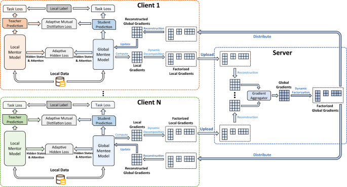

The local data is used to train the local mentor model and global mentee model. Both models are learned from local labeled data as well as the prediction and hidden results of each other. The local gradients are decomposed before uploading to the server, and then reconstructed on the server for aggregation. The aggregated global gradients are further decomposed and distributed to clients for local updates.

In our approach, we use three loss functions to learn mentee and mentor models locally, including an adaptive mutual distillation loss to transfer knowledge from output soft labels, an adaptive hidden loss to distill knowledge from the hidden states and self-attention heatmaps, and a task loss to directly provide task-specific supervision for learning the mentor and mentee models. We denote the soft probabilities of a sample xi predicted by the local mentor and mentee on the ith client as ({{{{{{{{bf{y}}}}}}}}}_{i}^{t}) and ({{{{{{{{bf{y}}}}}}}}}_{i}^{s}), respectively. Since incorrect predictions from the mentor/mentee model may mislead the other one in the knowledge transfer, we propose an adaptive method to weight the distillation loss according to the quality of predicted soft labels. We first use the task labels to compute the task losses for the mentor and mentee models (denoted as ({{{{{{{{mathcal{L}}}}}}}}}_{t,i}^{t}) and ({{{{{{{{mathcal{L}}}}}}}}}_{s,i}^{s})). We denote the gold label of xi as yi, and the task losses are formulated as follows:

$${{{{{{{{mathcal{L}}}}}}}}}_{t,i}^{t}={{{{{{{rm{CE}}}}}}}}({{{{{{{{bf{y}}}}}}}}}_{i},{{{{{{{{bf{y}}}}}}}}}_{i}^{t}),$$

(1)

$${{{{{{{{mathcal{L}}}}}}}}}_{s,i}^{t}={{{{{{{rm{CE}}}}}}}}({{{{{{{{bf{y}}}}}}}}}_{i},{{{{{{{{bf{y}}}}}}}}}_{i}^{s}),$$

(2)

where the binary function ({{{{{{{rm{CE}}}}}}}}({{{{{{{bf{a}}}}}}}},{{{{{{{bf{b}}}}}}}})=-{sum }_{i}{{{{{{{{bf{a}}}}}}}}}_{i}log ({{{{{{{{bf{b}}}}}}}}}_{i})) stands for cross-entropy. The adaptive distillation losses for both mentor and mentee models (denoted as ({{{{{{{{mathcal{L}}}}}}}}}_{t,i}^{d}) and ({{{{{{{{mathcal{L}}}}}}}}}_{s,i}^{d})) are formulated as follows:

$${{{{{{{{mathcal{L}}}}}}}}}_{t,i}^{d}=frac{{{{{{{{rm{KL}}}}}}}}({{{{{{{{bf{y}}}}}}}}}_{i}^{s},{{{{{{{{bf{y}}}}}}}}}_{i}^{t})}{{{{{{{{{mathcal{L}}}}}}}}}_{t,i}^{t}+{{{{{{{{mathcal{L}}}}}}}}}_{s,i}^{t}},$$

(3)

$${{{{{{{{mathcal{L}}}}}}}}}_{s,i}^{d}=frac{{{{{{{{rm{KL}}}}}}}}({{{{{{{{bf{y}}}}}}}}}_{i}^{t},{{{{{{{{bf{y}}}}}}}}}_{i}^{s})}{{{{{{{{{mathcal{L}}}}}}}}}_{t,i}^{t}+{{{{{{{{mathcal{L}}}}}}}}}_{s,i}^{t}},$$

(4)

where KL means the Kullback–Leibler divergence, i.e., ({{{{{{{rm{KL}}}}}}}}({{{{{{{bf{a}}}}}}}},{{{{{{{bf{b}}}}}}}})=-{sum }_{i}{{{{{{{{bf{a}}}}}}}}}_{i}log ({{{{{{{{bf{b}}}}}}}}}_{i}/{{{{{{{{bf{a}}}}}}}}}_{i})). In this way, the distillation intensity is weak if the predictions of mentor and mentee are not reliable, i.e., their task losses are large. The distillation loss becomes dominant if the mentee and mentor are well tuned (small task losses), which has the potential to mitigate the risk of overfitting. In addition, previous works have validated that transferring knowledge between the hidden states37 and hidden attention matrices38 (if available) is beneficial for mentee teaching. Thus, taking language model distillation as an example, we also introduce additional adaptive hidden losses to align the hidden states and attention heatmaps of the mentee and the local mentors. The losses for the mentor and mentee models (denoted as ({{{{{{{{mathcal{L}}}}}}}}}_{t,i}^{h}) and ({{{{{{{{mathcal{L}}}}}}}}}_{s,i}^{h})) are formulated as follows:

$${{{{{{{{mathcal{L}}}}}}}}}_{t,i}^{h}={{{{{{{{mathcal{L}}}}}}}}}_{s,i}^{h}=frac{{{{{{{{rm{MSE}}}}}}}}({{{{{{{{bf{H}}}}}}}}}_{i}^{t},{{{{{{{{bf{W}}}}}}}}}_{i}^{h}{{{{{{{{bf{H}}}}}}}}}^{s})+{{{{{{{rm{MSE}}}}}}}}({{{{{{{{bf{A}}}}}}}}}_{i}^{t},{{{{{{{{bf{A}}}}}}}}}^{s})}{{{{{{{{{mathcal{L}}}}}}}}}_{t,i}^{t}+{{{{{{{{mathcal{L}}}}}}}}}_{s,i}^{t}},$$

(5)

where MSE stands for the mean squared error, ({{{{{{{{bf{H}}}}}}}}}_{i}^{t}), ({{{{{{{{bf{A}}}}}}}}}_{i}^{t}), Hs, and As respectively denote the hidden states and attention heatmaps in the ith local mentor and the mentee, and ({{{{{{{{bf{W}}}}}}}}}_{i}^{h}) is a learnable linear transformation matrix. Here we propose to control the intensity of the adaptive hidden loss based on the prediction correctness of the mentee and mentor. Besides, motivated by the task-specific distillation framework in44, we also learn the mentee model based on the task-specific labels on each client. Thus, on each client the unified loss functions for computing the local update of mentor and mentee models (denoted as ({{{{{{{{mathcal{L}}}}}}}}}_{t,i}) and ({{{{{{{{mathcal{L}}}}}}}}}_{s,i})) are formulated as follows:

$${{{{{{{{mathcal{L}}}}}}}}}_{t,i}={{{{{{{{mathcal{L}}}}}}}}}_{t,i}^{d}+{{{{{{{{mathcal{L}}}}}}}}}_{t,i}^{h}+{{{{{{{{mathcal{L}}}}}}}}}_{t,i}^{t},$$

(6)

$${{{{{{{{mathcal{L}}}}}}}}}_{s,i}={{{{{{{{mathcal{L}}}}}}}}}_{s,i}^{d}+{{{{{{{{mathcal{L}}}}}}}}}_{s,i}^{h}+{{{{{{{{mathcal{L}}}}}}}}}_{s,i}^{t},$$

(7)

The mentee model gradients gi on the ith client can be derived from ({{{{{{{{mathcal{L}}}}}}}}}_{s,i}) via ({{{{{{{{bf{g}}}}}}}}}_{i}=frac{partial {{{{{{{{mathcal{L}}}}}}}}}_{s,i}}{partial {{{Theta }}}^{s}}), where Θs is the parameter set of mentee model. The local mentor model on each client is immediately updated by their local gradients derived from the loss function ({{{{{{{{mathcal{L}}}}}}}}}_{t,i}).

Afterwards, the local gradients gi on each client will be uploaded to the central server for global aggregation. Since the raw model gradients may still contain some private information45, we encrypt the local gradients before uploading. The server receives the local mentee model gradients from different clients and uses a gradient aggregator (we use the FedAvg method) to synthesize the local gradients into a global one (denoted as g). The server further delivers the aggregated global gradients to each client for a local update. The client decrypts the global gradients to update its local copy of the mentee model. This process will be repeated until both the mentee model and the mentor model converge. Note that in the test phase, the mentor model is used for label inference.

Algorithm 1

FedKD

Dynamic gradients approximation

In our FedKD framework, although the size of mentee model updates is smaller than the mentor models, the communication cost can still be relatively high when the mentee model is not tiny. Thus, we explore to further compress the gradients exchanged among the server and clients to reduce computational cost. Motivated by the low-rank properties of model parameters46, we use SVD to factorize the local gradients into smaller matrices before uploading them. The server reconstructs the local gradients by multiplying the factorized matrices before aggregation. The aggregated global gradients are further factorized, which are distributed to the clients for reconstruction and model update. More specifically, we denote the gradient ({{{{{{{{bf{g}}}}}}}}}_{i}in {{mathbb{R}}}^{Ptimes Q}) as a matrix with P rows and Q columns (we assume P ≥ Q). It is approximately factorized into the multiplication of three matrix, i.e., gi ≈ Ui∑iVi, where ({{{{{{{{bf{U}}}}}}}}}_{i}in {{mathbb{R}}}^{Ptimes K}), ({sum }_{i}in {{mathbb{R}}}^{Ktimes K}), ({{{{{{{{bf{V}}}}}}}}}_{i}in {{mathbb{R}}}^{Ktimes Q}) are factorized matrices and K is the number of retained singular values. If the value of K satisfies PK + K2 + KQ < PQ, the size of the uploaded and downloaded gradients can be reduced. Note that we formulate gi as a single matrix for simplicity. In practice, different parameter matrices in the model are factorized independently, and the global gradients on the server are factorized in the same way. We denote the singular values of gi as [σ1, σ2, . . . , σQ] (ordered by their absolute values). To control the approximation error, we use an energy threshold T to decide how many singular values are kept, which is formulated as follows:

$$mathop{min }limits_{K},frac{mathop{sum }nolimits_{i = 1}^{K}{sigma }_{i}^{2}}{mathop{sum }nolimits_{i = 1}^{Q}{sigma }_{i}^{2}}, > ,T.$$

(8)

To better help the model converge, we propose a dynamic gradient approximation strategy by using a dynamic value of T. The function between the threshold T and the percentage of training steps t is formulated as follows:

$$T(t)={T}_{{{{{{{{rm{start}}}}}}}}}+({T}_{{{{{{{{rm{end}}}}}}}}}-{T}_{{{{{{{{rm{start}}}}}}}}})t,tin [0,1],$$

(9)

where Tstart and Tend are two hyperparameters that control the start and end values of T. In this way, the mentee model is learned on roughly approximated gradients at the beginning, while learned on more accurately approximated gradients when the model gets to convergence, which can help learn a more accurate mentee model.

To help readers better understand how FedKD works, we summarize the entire workflow of FedKD (Algorithm 1).

Complexity analysis

In this section, we present some analysis on the complexity of our FedKD approach in terms of computation and communication cost. We denote the number of communication rounds as R and the average data size of each client as D. Thus, the computational cost of directly learning a large model (the parameter set is denoted as Θt) in a federated way is O(RD∣Θt∣), and the communication cost is O(R∣Θt∣) (we assume the cost is linearly proportional to model sizes). In FedKD, the communication cost is O(R∣Θs∣/ρ) (ρ is the gradient compression ratio), which is much smaller because ∣Θs∣ ≪ ∣Θt∣ and ρ > 1. The computational cost contains three parts, i.e., local mentor model learning, mentee model learning and gradient compression/reconstruction, which are O(RD∣Θt∣), O(RD∣Θs∣) and O(RPQ2), respectively. The total computational cost of FedKD is O(RD∣Θt∣ + RD∣Θs∣ + RPQ2). In practice, compared with the standard FedAvg4 method, the extra computational cost of learning the mentee model in FedKD is much smaller than learning the large mentor model, and SVD can also be very efficiently computed in parallel. Thus, FedKD is much more communication-efficient than the standard FedAvg method and meanwhile does not introduce much computational cost.

Reporting summary

Further information on research design is available in the Nature Research Reporting Summary linked to this article.

Source