
In the previous post, we discussed how Deep Q-Networks has proven to be a powerful tool for solving RL-based problems. However, over the years, several modifications to it have resulted in a great performance. In this article, I’ll discuss one of these modifications known as Double Deep Q-Networks (DDQN).
Overestimation in Q-learning
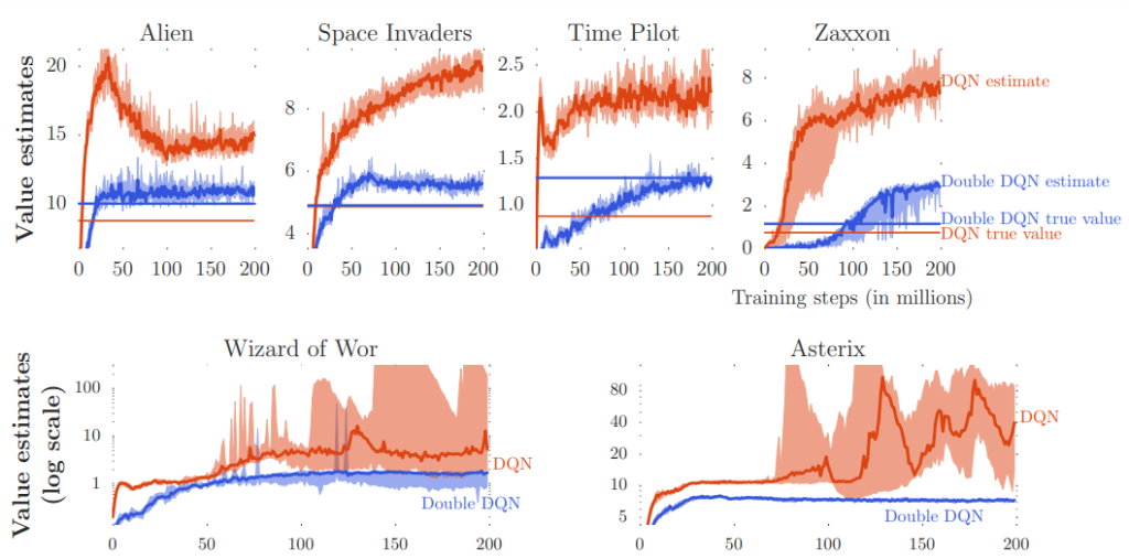
One of the challenges in Q-learning is that the Q function is updated based on estimates of the future rewards, rather than the true rewards. This can lead to an overestimation of the Q values, especially when the estimates are made using an inaccurate model of the environment. In other words, the agent may think it would get a higher reward than it actually would, leading to wrong decisions.
There are various techniques have been developed to address the problem of overestimation in Q-learning. One such technique is Double DQN.
Introduction to Double DQN
Value estimates of DDQN vs DQN
Double DQN is a variant of the deep Q-network (DQN) algorithm that addresses the problem of overestimation in Q-learning. It was introduced in 2015 by Hado van Hasselt et al. in their paper “Deep Reinforcement Learning with Double Q-Learning”.
In traditional DQN, the Q function is updated using the Bellman equation, which involves estimating the maximum expected future reward for each action. However, this can lead to the overestimation of the Q values, as described in the previous subtopic. On the other hand, DDQN addresses this problem by separating the action selection and action evaluation steps in the Q-learning update.
Specifically, in DDQN, the action with the maximum Q value is selected using one network (the “selection network”), and the Q value for this action is evaluated using a separate network (the “target network”).
Performance of DDQN
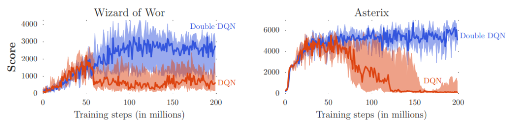 Performance of DDQN vs DQN
Double DQN has been evaluated on a variety of reinforcement learning tasks and has been shown to improve performance on many of them. In the original paper, the authors demonstrated improved performance on the Atari 2600 game suite compared to traditional DQN.
Additionally, other studies have also found that DDQN can lead to improved performance on tasks such as playing the card game Hanabi, controlling a simulated robot arm, and navigating a simulated 3D environment. In general, DDQN has been found to be particularly effective at reducing the overestimation of the Q values and improving the stability of learning.
However, Double DQN is not a panacea and may not always lead to improved performance. In fact, some studies have found that DDQN can perform worse than traditional DQN on certain tasks, such as playing the game of Go. Therefore, it is important to carefully evaluate the performance of DDQN on each specific task to determine whether it is likely to be beneficial. A comprehensive list of results performed by the authors of the DDQN paper is available on page 10 of the paper.
In summary, DDQN has been shown to improve performance on many reinforcement learning tasks, but it is not always the best choice and its effectiveness can vary depending on the specific task.
Implementation of DDQN
import torch import torch.nn as nn import torch.optim as optim import torch.nn.functional as F import numpy as np import random # Define the network architecture class QNetwork(nn.Module): def __init__(self, state_size, action_size): super(QNetwork, self).__init__() self.fc1 = nn.Linear(state_size, 64) self.fc2 = nn.Linear(64, 64) self.fc3 = nn.Linear(64, action_size) def forward(self, x): x = torch.relu(self.fc1(x)) x = torch.relu(self.fc2(x)) x = self.fc3(x) return x # Define the replay buffer class ReplayBuffer: def __init__(self, capacity): self.capacity = capacity self.buffer = [] self.index = 0 def push(self, state, action, reward, next_state, done): if len(self.buffer) < self.capacity: self.buffer.append(None) self.buffer[self.index] = (state, action, reward, next_state, done) self.index = (self.index + 1) % self.capacity def sample(self, batch_size): batch = np.random.choice(len(self.buffer), batch_size, replace=False) states, actions, rewards, next_states, dones = [], [], [], [], [] for i in batch: state, action, reward, next_state, done = self.buffer[i] states.append(state) actions.append(action) rewards.append(reward) next_states.append(next_state) dones.append(done) return ( torch.tensor(np.array(states)).float(), torch.tensor(np.array(actions)).long(), torch.tensor(np.array(rewards)).unsqueeze(1).float(), torch.tensor(np.array(next_states)).float(), torch.tensor(np.array(dones)).unsqueeze(1).int() ) def __len__(self): return len(self.buffer) # Define the Double DQN agent class DDQNAgent: def __init__(self, state_size, action_size, seed, learning_rate=1e-3, capacity=1000000, discount_factor=0.99, tau=1e-3, update_every=4, batch_size=64): self.state_size = state_size self.action_size = action_size self.seed = seed self.learning_rate = learning_rate self.discount_factor = discount_factor self.tau = tau self.update_every = update_every self.batch_size = batch_size self.steps = 0 self.qnetwork_local = QNetwork(state_size, action_size) self.qnetwork_target = QNetwork(state_size, action_size) self.optimizer = optim.Adam(self.qnetwork_local.parameters(), lr=learning_rate) self.replay_buffer = ReplayBuffer(capacity) self.update_target_network() def step(self, state, action, reward, next_state, done): # Save experience in replay buffer self.replay_buffer.push(state, action, reward, next_state, done) # Learn every update_every steps self.steps += 1 if self.steps % self.update_every == 0: if len(self.replay_buffer) > self.batch_size: experiences = self.replay_buffer.sample(self.batch_size) self.learn(experiences) def act(self, state, eps=0.0): device = torch.device(“cuda” if torch.cuda.is_available() else “cpu”) state = torch.from_numpy(state).float().unsqueeze(0).to(device) self.qnetwork_local.eval() with torch.no_grad(): action_values = self.qnetwork_local(state) self.qnetwork_local.train() # Epsilon-greedy action selection if random.random() > eps: return np.argmax(action_values.cpu().data.numpy()) else: return random.choice(np.arange(self.action_size)) def learn(self, experiences): states, actions, rewards, next_states, dones = experiences # Get max predicted Q values (for next states) from target model Q_targets_next = self.qnetwork_target(next_states).detach().max(1)[0].unsqueeze(1) # Compute Q targets for current states Q_targets = rewards + self.discount_factor * (Q_targets_next * (1 – dones)) # Get expected Q values from local model Q_expected = self.qnetwork_local(states).gather(1, actions.view(-1, 1)) # Compute loss loss = F.mse_loss(Q_expected, Q_targets) # Minimize the loss self.optimizer.zero_grad() loss.backward() self.optimizer.step() # Update target network self.soft_update(self.qnetwork_local, self.qnetwork_target) def update_target_network(self): # Update target network parameters with polyak averaging for target_param, local_param in zip(self.qnetwork_target.parameters(), self.qnetwork_local.parameters()): target_param.data.copy_(self.tau * local_param.data + (1.0 – self.tau) * target_param.data) def soft_update(self, local_model, target_model): for target_param, local_param in zip(target_model.parameters(), local_model.parameters()): target_param.data.copy_(self.tau * local_param.data + (1.0 – self.tau) * target_param.data)
Explanation
QNetwork: a PyTorch module that defines the architecture of the Q-network. It takes in a state and outputs the action values for all actions.
ReplayBuffer: a class that stores experiences in a circular buffer and samples a batch of experiences randomly for learning.
DDQNAgent: the main class that implements the Double DQN algorithm. It has the following methods:
__init__: initializes the local and target Q-networks, the optimizer, the replay buffer, and some hyperparameters. It also calls update_target_network to initialize the target network with the same weights as the local network.
step: stores an experience in the replay buffer and learns from a batch of experiences every update_every steps.
act: selects an action using an epsilon-greedy policy based on the action values output by the local Q-network.
learn: performs a learning step using a batch of experiences. It computes the Q-targets using the local Q-network and the action values output by the target Q-network, and then minimizes the loss between the Q-targets and the expected Q-values using the local Q-network. It then updates the target Q-network using polyak averaging.
update_target_network: updates the target Q-network with polyak averaging.
soft_update: a helper function that updates the target Q-network with polyak averaging.
To use this Double DQN implementation, you can create an instance of the DDQNAgent class and call its act and step methods in your training loop. You can also customize the hyperparameters and the network architecture by modifying the __init__ method of the DDQNAgent class.
Training DDQN
 Cart Pole task from OpenAI Gym
Assuming we’ve saved the previous code snippet in a file called ddqn.py, the following snippet can be used to import and train the agent on performing the CartPole task:
import gym import numpy as np from ddqn import DDQNAgent import matplotlib.pyplot as plt # Create the environment env = gym.make(‘CartPole-v0′) # Get the state and action sizes state_size = env.observation_space.shape[0] action_size = env.action_space.n # Set the random seed seed = 0 # Create the DDQN agent agent = DDQNAgent(state_size, action_size, seed) # Set the number of episodes and the maximum number of steps per episode num_episodes = 1000 max_steps = 1000 # Set the exploration rate eps = eps_start = 1.0 eps_end = 0.01 eps_decay = 0.995 # Set the rewards and scores lists rewards = [] scores = [] # Run the training loop for i_episode in range(num_episodes): print(f’Episode: {i_episode}’) # Initialize the environment and the state state = env.reset()[0] score = 0 # eps = eps_end + (eps_start – eps_end) * np.exp(-i_episode / eps_decay) # Update the exploration rate eps = max(eps_end, eps_decay * eps) # Run the episode for t in range(max_steps): # Select an action and take a step in the environment action = agent.act(state, eps) next_state, reward, done, trunc, _ = env.step(action) # Store the experience in the replay buffer and learn from it agent.step(state, action, reward, next_state, done) # Update the state and the score state = next_state score += reward # Break the loop if the episode is done or truncated if done or trunc: break print(f”tScore: {score}, Epsilon: {eps}”) # Save the rewards and scores rewards.append(score) scores.append(np.mean(rewards[-100:])) # Close the environment env.close() plt.ylabel(“Score”) plt.xlabel(“Episode”) plt.plot(range(len(rewards)), rewards) plt.plot(range(len(rewards)), scores) plt.legend([‘Reward’, “Score”]) plt.show()
The progress of training may look like the following:
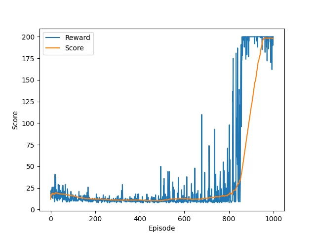 DDQN training
Final Thoughts
That’s it! Hope you found this helpful. Let me know if there are any questions in the comments below. Also, feel free to check out my other posts on Reinforcement Learning here.